Demystifying Level of Detail Expressions

Believe it or not, to really understand the mechanics of Level of Detail expressions / LoD calculations, you just need to look at Grand Totals.

What does a Grand Total do? It takes aggregates already in your view and applies another aggregation on top of them to give you a second aggregate.

For example, after enabling Grand Totals, you can go to Analysis > Totals > Total All Using and select a second aggregation. You can take all the aggregate values in your view and find the overall average, the maximum, the minimum, etc. You get the picture.

LoDs perform the same function, except they bypass the view itself. They do not require you to first place dimensions into the view so that aggregates can be generated, because they do not require these view level aggregates in order to apply a second aggregation.

Two Levels of Aggregation:

Any aggregation you wrap around a measure in your view is calculated at row level. For example, AVG([Sales]) takes the “Sales” value from every single row and returns the overall average.

When you add a dimension to your view, results are still calculated at row level; the results are simply partitioned across the members of the dimension in your view, producing multiple aggregates instead of one. But the averages themselves are still calculated on a row-by-row basis.

The way the aggregation is computed is the same, but the aggregates that result are defined by the members of the dimensions in your view. Tableau’s official name for the view level of detail is ”Viz Level of Detail” or “Viz LoD”.

Therefore, row level aggregation (which we’ll refer to as the ‘first’ aggregation from now on) gives us our Viz level aggregates (as determined by the ‘Viz LoD’).

The ‘second’ aggregation is computed using these viz level aggregates to give us our higher level aggregates, such as Grand Totals.

Grand Totals, Table Calculations, and Reference Lines are probably the only standard features of Tableau that let you apply a second aggregation to already aggregated values.

LoDs essentially follow the same logic, but by creating a ‘phantom’ Viz LoD that generates the relevant Viz level aggregates behind the scenes. This way, you don’t need to place these dimensions into the view first, like you do when using Tableau’s Grand Totals feature.

LoDs have the benefit of being like any other measure in the dataset; but one that has already computed at row level and partitioned aggregates according to the relevant dimensions, so that when you bring it into a view, you can apply the ‘second’ aggregation straight away by wrapping it inside an aggregate function.

You’re able to do this because, despite the underlying partitioning happening behind the scenes, LoDs result in non-aggregate values, just like a native field included in the data set. You can wrap them in any aggregate function, like SUM(), AVG(), etc., or even the ATTR() function if you want to, just like any other measure.

Let’s say you wanted to know the average sales value per order. You could use SUM([Sales]) / COUNTD([Order ID]). The problem is that your result would be an aggregate value, or AGG(). So if you wanted to know the maximum sales value per order, you wouldn’t be able to use a MAX() aggregation with this logic to find the max sum of sales per order because this logic gives you a single, high level result.

But a LoD, on the other hand, can give you the order level sales value as a brand new field that is non-aggregated, so you can then wrap it inside the MAX() function to get the highest sales at the order level. It is the literal equivalent of using a GROUP BY clause in SQL to create a new measure that gives you a total aggregation at a higher level of detail than row level.

Now let’s move on to the keywords that make up the three types of LoDs.

The Mechanics of Level of Detail Expressions

LoD expressions are made up of the following syntax, which is comprised of three parts:

All LoDs start and end with curly braces.

Before the colon, you have the first two parts of the syntax. You first specify the keyword (FIXED, INCLUDE, or EXCLUDE) and then you specify the “Dimension Declaration”, which is where we define our ‘phantom Viz LoD’. So this is where you define the level of detail you’d like to use behind the scenes. You can also think of this as the “GROUP BY” part of the SQL statement.

After the colon, you define the type of row level aggregation (first aggregation) that you want to assign to this ‘phantom Viz LoD’. Again, just picture this as if it were a view that you were building. If you want to know the max sales value per order, you would first need to know the SUM([Sales]) per order. So in the Dimension Declaration, you’d list [Order ID], and in the Aggregate Expression, you’d list SUM([Sales]).

Let’s stick with the INCLUDE keyword for now, but I will elaborate on each keyword’s individual use shortly. The LoD expression we would need to answer our question would look like this: { INCLUDE [Order ID] : SUM([Sales]) }

To get the highest value, you would simply wrap the LoD calculation in a MAX() function. This would give you the exact same result as building a view with the same measure and dimension, enabling Grand Totals and setting “Total All Using” to “Maximum”.

It’s that simple.

In a nutshell, the LoD is calculating the first aggregation (row level aggregation) and partitioning the results to a higher level defined in the “Dimension Declaration” behind the scenes, thereby allowing you to apply the second aggregation simply by wrapping it inside a standard aggregation.

FYI, where Grand Totals only offer you a limited set of “second aggregations”, LoDs allow for the following: SUM, AVG, MIN, MAX, MEDIAN, COUNT, COUNTD, VAR, VARP, STDEV, STDEVP, PERCENTILE, COVAR, COVARP, COLLECT, and CORR.

Obviously, a huge benefit of LoDs is that you can use them in different ways, just like with any other measure. Unlike Grand Totals or Reference Lines, you are not limited to how you can visually portray them. You can create bar charts or literally anything else that’s within the scope of Tableau’s possibilities.

LoD Keywords (Include and Exclude)

With the understanding that LoD expressions create a ‘phantom’ view to generate results, let’s take a look at how the keywords work.

INCLUDE does exactly what we’ve described above. It includes the dimensions from the Dimension Declaration into the Viz LoD, but ‘invisibly’, so that the aggregation we wrap it in (the second aggregation) is aggregating the aggregates that would hypothetically be in the view if those dimensions were added to the view directly.

Therefore, in our example above, no matter what actual dimensions we add to our view or Viz LoD, the LoD itself includes [Order ID] behind the scenes as well. And so, when we wrap it in a second aggregation, like AVG(), it will return the order level average and not the row level average.

An EXCLUDE LoD uses the Dimension Declaration to target / pin-point dimensions already in the Viz LoD and then pretends they’re not there when calculating results. Think of when you set a Reference Line to ‘entire window’ instead of ‘cell’; it will ignore some of the dimensions in the view to give you a higher level value. Likewise, an EXCLUDE LoD lets you specify which of those dimensions you want to ignore. This means that the second aggregation will only be applied across remaining dimensions in the view, similar to how a Reference Line works.

And of course, you can use the EXCLUDE LoD to build any view you want, as it is not limited to Reference Lines.

LoD Keywords (Fixed)

Before we move onto the final keyword, you first need to understand the two types of relationships that exist between dimension members in a data set.

One-to-many relationships exist where there is a clear hierarchy. A city can only belong to one state; a state can only belong to one country; and so on and so forth.

Many-to-many relationships exist when there is no clear hierarchy and members are ‘shared’. For example, YEAR([Order Date]) can be associated with multiple cities, and a city can be associated with multiple years.

You can tell whether there is a clear hierarchy by placing two dimensions next to each other on the Rows shelf. Place them in any order and note the structure of the layout, then swap the order around.

If multiple members exist to the right of the first dimension only once but result in a row level table in the opposite scenario, the dimensions have a clear hierarchy and therefore have a one-to-many relationship with each other.

If multiple members exist to the right of the first dimension, no matter the order of the fields, then the two dimensions have a many-to-many relationship with each other.

There are a few exceptions, such as “Apple Valley”, which is a city in our data set. These are two different cities belonging to different states that share the same name. So in theory, there is still a clear hierarchy because they are technically two different cities. But in terms of the data set, this particular “city” will have a many-to-many relationship with “state”, while the majority of cities will have a many-to-one or hierarchical relationship with “state”.

With that covered, let’s move on to FIXED LoDs. A FIXED LoD says, “Pretend these dimensions in the Dimension Declaration are the ONLY dimensions in the Viz LoD when computing behind the scenes”. From that point onward, the relationship between dimensions in the view and dimensions in the Dimension Declaration comes into play.

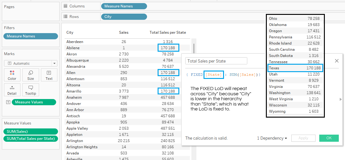
If the dimensions used in the actual Viz LoD have a one-to-many relationship with the dimensions declared in the Dimension Declaration and are lower in the hierarchy order, then the LoD value will repeat across each member of that dimension because the LoD is fixed to a higher level of detail.

For example, a FIXED LoD set to “State” but displayed in a view only showing “City” will only show the higher, state level value associated with that city.

The only exception would be for a city like “Apple Valley”, where the value would be higher than expected, but only because there are two “Apple Valleys” in the data set. Therefore, the value shown will be the sum of the two different state level values.

If the dimensions in the view are higher in the hierarchy, then obviously the FIXED LoD will roll up because the LoD is fixed to a lower level of detail, which means it will work just like a traditional measure that aggregates and rolls up to the dimensions in the view.

If the dimensions in the view have a many-to-many relationship with those used in the Dimension Declaration, they will be ignored, and the LoD’s result will repeat across them. Why? Think of a GROUP BY clause. If you set the level of detail in your clause to “City” only, then you would end up with total aggregates for each member of “City”, regardless of what date or year you’re looking at in the data set.

If YEAR([Order Date]) was also included in the clause, only then would the values reflect the different values for both “Year” and “City”.

If, however, you were viewing the data at state level, the results of the GROUP BY statement would still be able to roll up because “State” is higher in the one-to-many or hierarchical relationship.

Smart Aggregations

Using our example from earlier: { FIXED [Sub-Category] : SUM([Sales]) }, if you were to actually view the underlying data, you would find the output of this FIXED LoD repeated across all lower levels of detail, just as we’ve seen above when a dimension with a lower level of detail is added to the view.

But despite this, Tableau is smart enough to know not to count each instance of that value when rolling up, but instead counts each sub-category-level value only once.

This is a major advantage over using the GROUP BY clause in SQL, because if added to our data set via that method, every underlying instance of that value would result in multiplication because, by default, all native fields are aggregated at row level.

But with LoDs, Tableau knows to aggregate only at the level you’ve defined in the Dimension Declaration. So if you define “Sub-Category” as the level, it will count each sub-category’s value only once.

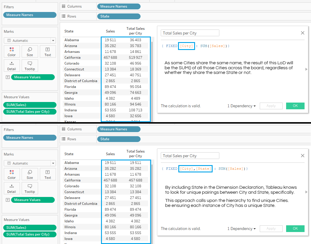
If you were to try something similar using { FIXED [City] : SUM( [Sales]) }, you may notice that some values appear higher than expected.

This comes back to the issue we had before, whereby you have multiple cities that share the same name. So when you fix a LoD at city level, you are fixing the sum of all cities that share that name, regardless of whether they share the same state or not.

To avoid mass amalgamation, you can add the dimension that is immediately above “City” in the hierarchy order—which is “State” in our case—to the Dimension Declaration. Now, the fixed results will not only be at city level, but will respect the city and state hierarchy because they look for unique pairings between them.

Why Use FIXED LoDs At All?

It is easy to see that with the right mix of dimensions inside the Dimension Declaration, a FIXED LoD could technically be used to achieve the same results as either an INCLUDE or an EXCLUDE LoD. Why, then, would we use FIXED LoDs?

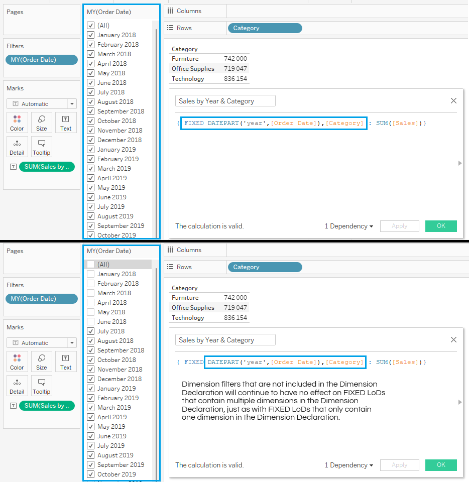
There are two main reasons. The first has to do with filters. If we look at Tableau’s Order of Operations list, it shows the order in which background functions take place. Note how FIXED LoDs come into effect immediately after Extract, Data Source and Context Filters. Dimension Filters only come into play afterwards, followed by INCLUDE and EXCLUDE LoDs.

What this means is that results generated from FIXED LoDs are based on all the data that exists in a data set. Dimension Filters that are applied in the view will not affect the results.

The only time a Dimension Filter made using a dimension not in the Dimension Declaration will appear to have an impact on the outcomes is if the values that are filtered out happen to filter out absolutely all rows associated with a member of the dimension used in the Dimension Declaration. It would have the same effect as using the actual dimension used in the Dimension Declaration as the filter and filtering out one of its members.

Likewise, filtering out a member in a dimension higher up in a one-to-many hierarchy with the dimension used in the Dimension Declaration will make all underlying data points disappear from view.

For scenarios where the dimension used in the Dimension Declaration is not actually in the view itself, it is the aggregate or total value that will be affected in the view. For example, filtering out "Furniture" directly affects all Sub-Categories within "Furniture" due to its one-to-many relationship with Sub-Category, therefore the LoD’s value will be affected.

If you add both “Category” and “Sub-Category” to the Dimension Declaration and filter out members of the lower dimension in the hierarchy—which is “Sub-Category” in this case—then the results of the LoD will be affected because of the one-to-many relationship.

Filtering by “Category”, which is higher in the hierarchy, would simply remove the data point from view, as we’ve already learned.

Even if dimensions with a many-to-many relationship were used in the Dimension Declaration, the results of the LoD would be affected if filtered by them. In this case, it would be affected whether you use one or the other because of their many-to-many relationship.

Just as before, filtering by dimensions not mentioned in the Dimension Declaration will have no effect on the LoD result, unless you filter out all data points relating to a member of a dimension that is mentioned in the Dimension Declaration.

So that is how filtering works with FIXED LoDs. When it comes to INCLUDE and EXCLUDE LoDs, they are calculated using values that remain after applying Dimension Filters.

Likewise, according to our Order of Operations table, we can see that Measure Filters and Table Calculation Filters will not have an effect on INCLUDE and EXCLUDE LoDs.

You can, however, “bend the rules” when you right-click on a Dimension Filter and select “Add to context”. This changes it from a Dimension Filter to a Context Filter. Along with this change comes a change in behavior in FIXED LoDs.

Now the filter no longer comes after FIXED LoDs in the Order of Operations chart, but before. This means that when the user filters out a value, the result of the FIXED LoD’s first aggregation will now also be affected by this change.

It is natural to make the assumption that if a Dimension Filter added to context now affects a FIXED LoD, then the LoD will adapt to that dimension if it were also added to the view.

However, this is not true. The FIXED LoD will now take any filtered-out members of that dimension into account when calculating the results, but the FIXED LoD’s Dimension Declaration still defines the level of detail at which the values will be calculated. Therefore, it will still ignore and repeat across this dimension in the view, that is not part of the Dimension Declaration, even if that dimension is now added to context under filters.

Creating Dimensions using FIXED LoDs

But aside from being able to produce results that are not affected by Dimension Filters, another important reason FIXED LoDs are worthwhile is that they can be used to create brand new dimensions in your data set, whereas INCLUDE and EXCLUDE LoDs can only create new measures.

For example, you can create a new date field using { FIXED [Customer ID] : MIN([Order Date]) }. This would give you the earliest order date per customer.

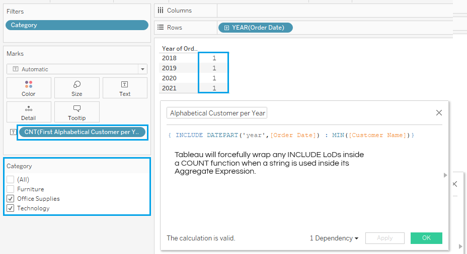
Likewise, { FIXED DATEPART('Year',[Order Date]) : MIN([Customer Name]) }, would give you the first alphabetical customer name per year, resulting in a string field.

Technically, you can create similar calculations using INCLUDE and EXCLUDE, but Tableau will force them into measures. Tableau will either wrap them in a COUNT function in the case of strings, or, in the case of dates, will only allow you to use the date as a continuous field. But traditional date options typically associated with a date field will not be available.

Even if you tried dragging the fields up into the dimensions pane, Tableau would not allow it.

But creating a dimension using a FIXED LoD is incredibly useful. You could find the first order per customer: { FIXED [Customer ID] : MIN([Order Date]) } and place this new date field onto rows, wrap it in a MONTH() aggregation, and drag COUNTD([Customer ID]) onto columns. This would show the number of onboarded customers by month, creating buckets or groupings just as with any other dimension, because FIXED LoDs that result in dates retain the traditional properties of a date field.

Additional Advantages of LoDs

LoDs can also be used inside other calculations, including other LoDs, just like any other field in the data set.

It is a brilliant solution to the ever-frustrating “Cannot mix aggregates and non-aggregate arguments with this function” error message that we all love to hate.

For example, [Order Date] = MAX([Order Date]) would result in that error, but we can fix that simply using [Order Date] = { FIXED : MAX([Order Date]) } because the results of LoDs are not aggregated.

If you want the MAX([Order Date]) to be relative to your filter selections, you need to apply what we discussed earlier and add the Dimension Filter to context. You will need to do this for every Dimension Filter that you want the FIXED LoD to take into account.

Table-Scoped LoDs

The Dimension Declaration used in LoDs is actually optional. By omitting the Dimension Declaration from a FIXED LoD altogether, you can produce a table-scoped LoD. So if we used {MIN([Order Date])}, we would be able to find the very first order date in the data set. Table-scoped LoDs are FIXED LoDs by default and can be written as either { Aggregate Expression } or { FIXED : Aggregate Expression }. Both options produce the same results.

The same would happen if we used { FIXED : SUM([Sales]) }. We would get the total sales across all rows.

Likewise, if we used { FIXED : MAX([Discount])}, we would get the largest row-level discount in our data set.

Table-scoped LoDs work similarly to EXCLUDE LoDs, whereby they have the ability to ignore any dimensions in the Viz LoD. The key difference, as we know, would be that the EXCLUDE LoD will still update based on filter selections and will still adapt to any additional dimensions that are brought into the Viz LoD, whereas the FIXED or table-scoped LoD would stay the same, unless a Dimension Filter is added to context.

Excluding the Dimension Declaration from an INCLUDE or EXCLUDE LoD would serve no purpose because this would result in a row-level calculation that adapts to other dimensions in the view, essentially achieving the same thing as standard, non-LoD measure.

Troubleshooting

It is important to understand that Tableau reads YEAR([Order Date) differently to DATEPART(‘year’, [Order Date]) when it comes to INCLUDE and EXCLUDE LoDs, even though we know they equate to the same thing.

Tableau doesn’t elaborate on why this is exactly, but to avoid any issues, they recommend dragging aggregated dates used in the Viz LoD into the Dimension Declaration directly instead of typing it out. This way, it will generate the correct syntax or formula required to match what is actually happening in the view.

This only seems to affect INCLUDE and EXCLUDE LoDs, but FIXED LoDs do not appear to have the same issue.

Another strange behavior among INCLUDE and EXCLUDE LoDs is that they cannot link logic with calculated fields, but they can link logic with logic or calculated field references with calculated fields.

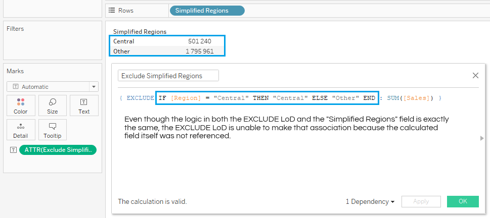
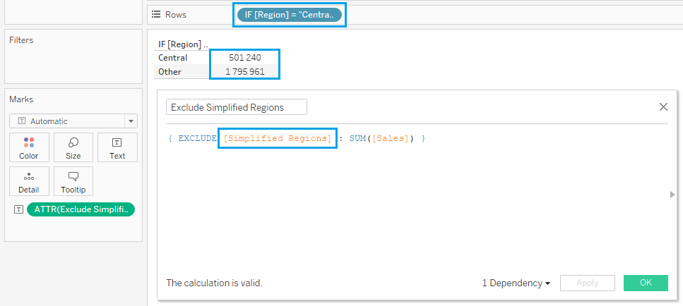
Let me explain: if you use the logic IF [Region] = "Central" THEN "Central" ELSE "Other" END inside the Dimension Declaration of an EXCLUDE LoD, but create a separate field with the same logic called “Simplified Regions”, then the EXCLUDE LoD will not be able to make the association between the logic it contains and the calculated field, even if you place that field into the Viz LoD.

The same is true in the reverse scenario.

You must either use the logic in both the LoD and the view, or the calculated field reference in both places.

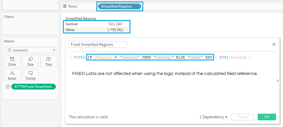
If you’re using an INCLUDE LoD, this doesn’t really matter because the LoD will still adapt to whatever is in the view any way. And just like before, a FIXED LoD is not affected by this issue.

Lastly, Aggregate Expressions must always be aggregates, and therefore, you cannot use an ATTR() function inside of a LoD.

This is true regarding the Dimension Declaration of a LoD as well.

And that’s finally it!

Since the introduction of the Relationships data model, LoDs have played an important role in getting different tables to talk to each other in the right way in order to show the results you want.

But that’s an entirely different use case for LoDs that would require a separate whitepaper. The mechanics, however, would remain the same.